Analysis of variance

When analysis of variance (ANOVA of English analysis of variance ) refers to a large group of data- analytical and structure -checking statistical procedures that allow for many different applications. They have in common that they compute variances and test statistics in order to gain insight into the stuck behind the data regularities. The variance of one or more target variable (s) is thereby explained by the influence of one or more predictor variables (factors). The simplest form of analysis of variance tests the influence of a single nominally scaled to a metrically scaled variables by comparing the mean values of the dependent variable within the plane defined by the categories of the independent variable groups. Thus, the analysis of variance in its simplest form, an alternative to the t-test is suitable for comparisons between more than two groups.

6.1 Example
6.2 Basic idea of the invoice
Table 6.3

Distinction

Depending on whether one or more target variables are present, there are two forms of analysis of variance:

The univariate analysis of variance, variance according to the English term analysis of referred to as ANOVA
The multivariate analysis of variance, multivariate analysis of variance according to the English name referred to as MANOVA

Depending on whether one or more factors are present, a distinction is made between einfaktorieller ( easier) and multifactorial ( multiple ) analysis of variance.

Terms

Target variable (dependent variable ) The metric random variable whose value is to be explained by the categorical variables. The dependent variable contains measurement values .

Predictor (factor; independent variable) The categorical variable ( = factor), which defines the groups. Their influence is to be checked, it is nominally scaled.
The categories of a factor then called factor levels. This term is not identical with that in the factor analysis.

The basic idea

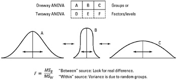
Inspect the process, whether (and if so, how ), the expectation values of the metric random variables in different groups differ (even classes). With the test values of the process it is checked whether the variance between groups is greater than the variance in the groups. This can be determined whether the grouping is useful or not, or whether the groups differ significantly or not.

If they differ significantly, it can be assumed that in the groups act different laws. Thus, for example, determine whether the behavior of a control group with an experimental group is identical. For example, if the variance of one of these groups already repaid on causes ( sources of variance ), it can be concluded at variance equality that in the other group, no new action cause (eg by the experimental conditions ) was come.

See also: discriminant analysis, coefficient of determination

Requirements

The use of any form of analysis of variance is tied to conditions, the existence of which must be checked before each calculation. Do not meet these requirements, the records, so the results are useless. The requirements are slightly different depending on the application, generally apply the following:

Homogeneity of variance of the sampling variables
Normal distribution of the sampling variables

The check is made with other tests outside of the analysis of variance, but these are now included as standard in statistics programs as an option. The normal distribution can be checked, for example, for each variable with the Shapiro -Wilk test. If these conditions are not met, distribution-free, nonparametric methods are available, which are robust, but have lower test strength.

Non-parametric methods: for two samples (t- test alternatives ): paired (dependent) Sp: Wilcoxon signed - rank test
Unpaired (independent) Sp: Mann-Whitney U test also known as the Wilcoxon-Mann -Whitney test, U - test, Mann -Whitney - Wilcoxon ( MWW ) test or Wilcoxon rank sum test.

Paired data: Friedman test, Quade test
Unpaired data: Kruskal -Wallis test, Jonckheere - Terpstra test, Umbrella Test
For multifactorial analysis: Scheirer - Ray -Hare test

One-Way ANOVA

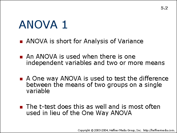
In a one-factor analysis of variance to examine the influence of an independent variable (factor) with k different levels ( groups) to the values of a random variable. To the k mean values of the expressions for the groups are compared with each other, and that one compares the variance between groups with the variance in the groups. Because make up the total variance from the two components mentioned, it is called analysis of variance. The one-way ANOVA is a generalization of the t-test in case more than two groups. For k = 2 is equivalent to the t-test.

Requirements

The error components must be normally distributed. Error components denote the respective variances (total, treatment and error variance). The validity of this assumption is at the same time requires a normal distribution of the measured values in the respective population.
The error variances must be between the groups (ie, the k factor levels ) is equal or homogeneous ( homoscedasticity ).
The measured values or factor levels must be independent of each other.

Example

This form of analysis of variance is appropriate when you want to, for example, investigated whether smoking has an effect on the aggressiveness. Smoking is here an independent variable, which ( k = 3 factor levels ) can be divided into three forms: Non smoking, smoking weak and heavy smokers. The detected through a questionnaire aggressiveness is the dependent variable. To carry out the study, the subjects are assigned to the three groups. After the questionnaire is submitted, with the aggression is detected.

Hypotheses

It is the expectation value of the dependent variable in the ith group. The null hypothesis of a one-factorial analysis of variance is:

The alternative hypothesis is:

The null hypothesis is therefore that between the expected values of the groups ( corresponding to the factor level or factor levels ) there is no difference. The alternative hypothesis states that there is a difference between at least two expected values . If we have for example five factor levels, then the alternative hypothesis is confirmed if differ at least two of the group means. However, it is also three expectation values or four or all five differ significantly from each other.

If the null hypothesis is rejected, the analysis of variance thus provides no information as to what factor or between stages is a difference between how many. We know then only with a certain probability (see significance level ) that at least two forms have a significant difference.

One can now ask whether it would be admissible in pairs to perform with various t-tests individual comparisons between means. Comparing with the analysis of variance only two groups (ie, two averages ), then perform t-test and analysis of variance to the same result. However, there are more than two groups, the review of the global null hypothesis of variance analysis of paired t-test is not allowed - it comes to the so-called alpha error accumulation. With the help of multiple comparison techniques can be checked after a significant ANOVA result, in which mean value of the pair or are the differences. Examples of such techniques are compared with the Bonferroni and the Scheffé test. The advantage of this method is that they take into account the aspect of alpha inflation.

Basic idea of the invoice

The calculation of the analysis of variance is first calculated the total variance observed in all groups. They are surrounded by it all the measured values from all groups together, calculated the overall mean value and the total variance.

Then you want the variance of the total variance, which goes back only to the factor determine. If the total observed variance went back to the factor, then have all measured values in a factor level be the same - then likely only differences between the groups exist. Since all measured values within a group have the same factor expression, they consequently have to have all the same value, since the factor would be the only varianzgenerierende source. In practice, also measured values within a factor level but differ. These differences within the groups must therefore come from other influences (either random or so-called confounders ).

Between the total variance and the variance Treatment usually a mismatch - the total variance is greater than the variance of Treatment. The variance, which is not due to a factor (the " treatment" ) are referred to as error variance. This is due either to chance or other, not investigated variables ( confounders ).

The ultimate test of significance is via a "normal " F- test. One can mathematically show that the analysis of variance is also valid if the null hypothesis that treatment and error variance must be equal. With an F test you can check the null hypothesis that two variances are equal, by forming the quotient of them.

Mathematical Model

The model in effect representation is:

It includes: Xij: the target variable; assumed to be normally distributed in the groups k: number of factor levels of the considered factor ni: sample sizes for the individual factor levels μ: arithmetic mean of the expected values in the groups? i: Effect of the i-th level of a factor εij: Interference, independent and normally distributed with mean 0 and the same ( unknown ) variance σ2.

For the expectation value in the ith group to write normally, and we have:

Sums of squares

The overall variability, QST, expressed as the total square deviation from the mean, can be broken down into two parts. A part refers to the group membership, and the other part, the rest is attributed to chance. The first part, QSA, lets be expressed as the quadratic error of the mean from the grand mean of the groups. The remainder, QSE, concerning the differences within the groups is expressed as the total variation of the mean values in the groups. Thus:

Therein:

And

The two sums of squares QSA and QSE are stochastically independent.

In the case of k groups with the same size n / k is valid under the null hypothesis also:

And

Test statistic

It usually defines also the mean sums of squares:

And

This makes it possible to define the test statistic as:

In the case of groups of the same size is F under the null hypothesis that is F- distributed with k- 1 degrees of freedom in the numerator and nk degrees of freedom in the denominator.

If the test statistic is significant, at least two groups differ from each other. In post- hoc tests can then be calculated between which each group is the difference.

Example calculation

The following example is a simple analysis of variance with two groups (also two-sample F- test). In an attempt to obtain two groups () of 10 () animals of different food. After some time their weight gain is measured with the following values :

It will be investigated whether the different food has a significant effect on the weight. The mean and the variance (in this case " estimate ", sample variance ) amount of the two groups

As can be calculated from:

And

The probabilistic model underlying assumes that the weights of the animals are normally distributed and have the same variance per group. The null hypothesis to be tested is

Obviously, the means are different and. However, this difference could also be within the range of natural variability. To check whether the difference is significant, the test statistic is calculated.

The size is according to the underlying model is a random variable with a distribution, with the number of groups ( factor levels ) and the number of measured values. The indices are referred to as degrees of freedom. The value of the F distribution for given degrees of freedom (F- quantile ) can be looked up in a Fisher - board. Here still a desired significance level must ( the probability of error ) can be specified. In the present case, the F- quantile is the probability of error of 5%. This means that for all values of the test statistic to 4.41, the null hypothesis can not be rejected. Since, the null hypothesis can be rejected at the present values.

It can therefore be assumed that the animals actually have a different weight in the agent in the two groups. The probability to take a difference, although this is not present, is less than 5%.

Two-Factor ANOVA

The two-factorial analysis of variance considered to explain the target variables, two factors (factor A and factor B).

Example

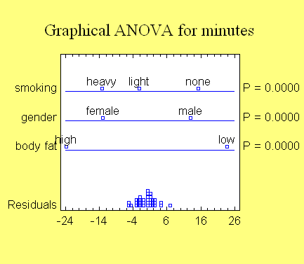
This form of analysis of variance is shown for example in studies who wish to represent the influence of smoking and drinking coffee on the nervousness. Smoking is here the factor A, which, for example, in three variants ( factor levels ) can be divided into: non- smokers, light smokers and heavy smoker. The factor B can be the daily amount of coffee used with the steps: 0 cups, 1-3 cups, 4-8 cups, more than 8 cups. The nervousness is the dependent variable. To carry out the study subjects are over 12 groups distributed according to the combinations of factor levels. The measurement of nervousness is performed, which provides metric data.

Basic idea of the invoice

The model (for the case with fixed effects ) is in effect representation:

It includes:

Interaction describes a particular effect, which occurs only when the combination of factor levels (i, j ) is present.

The total sum of squares QST is here divided into four independent parts.

It includes:

The expected values of the sums of squares are:

The sums of squares are divided by chi-square distributed under suitable assumptions, namely:

The mean sums of squares arise in Dividierung the sums of squares by their degrees of freedom

The true test statistics are calculated as the quotient of the mean sums of squares, with MQSeries as the denominator.

Now you calculate the variance for each factor, and the variance for the interaction of A and B. The null hypothesis H0 is that there is no interaction. Again, the hypothesis is calculated from the test statistic F. This is now combined as the quotient of the emerged by the interaction of A and B, and the error variance. Now One compares with the F- quantiles by specifying a desired significance level. If the test statistic F is greater than the quantile (the latter can be read in relevant tables), then H0 is rejected, so there is an interaction between the factors A and B.

Table

In a practical analysis of the results are summarized in a table:

Factorial ANOVA with more than two factors

Several factors are possible. However, the data required for estimation of the model parameters with the number of factors increases considerably. And the representations of the model ( for example, tables) are less clear as the number of factors. More than three factors can only be represented heavily.