Conditional probability

Conditional probability (including conditional probability ) is the probability of occurrence of an event under the condition ( also conditionality ) that the occurrence of another event is already known. It is written as. The vertical bar is read as " on condition " and be understood as follows: When the event occurred, the options are limited on the results. Thus, the probability changes; this new probability of the event is given by. The conditional probability can thus be interpreted as a re-assessment of the probability that, when the information is obtained, that the event has already occurred. Sometimes the notation is used, but may also have other meanings.

For a generalized, abstract concept of conditional probabilities see conditional expectations.

• 7.1 Examples with dice 7.1.1 Special Cases
• 7.1.2 General Case

Motivation and definition

Sometimes one would like to examine how strong the statistical influence of a size to another. For example, you want to know whether smoking () carcinogenic ( ) is. The logical implication would require that the conclusion is valid for all instances; So, that is that every smoker will have cancer. A single smoker who does not get cancer, would the sentence "Smoking causes cancer of calls with logical security. ", Or " Every smoker gets cancer. " ad absurdum. Nevertheless, although there are smokers without cancer, there is a statistical relationship between these two events: This connection is that the probability of developing cancer is increased in smokers. This probability is the conditional probability that someone gets cancer, with the proviso that it is smoking (). Stochastic probability may also be examined, that someone is smoking, with the proviso that it has cancer. In the theory of probability is therefore to note that the term of the condition is not tied to a causal or temporal relationship. The conditional probability is a measure of how strong the statistical influence of on. It can be viewed as a stochastic measure of how likely the final. But she says, like all statistical quantities, nothing on the possible causality of the relationship.

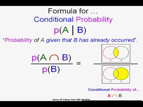
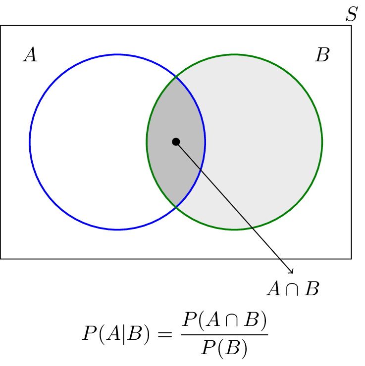
With this motivation we arrive at the following definition: If and are arbitrary events and, then, the conditional probability of A, provided B ( the probability of A under the condition B ) is listed as ( with vertical line between A and B), defined by:

This is the probability that and occur together. is called the joint probability, joint probability or average probability. denotes the set-theoretic intersection of the events and.

Multiplication sentence

Rearranging the definition formula of the multiplication theorem for two events occurs:

Generalization

Generalizing the above expression of the multiplication theorem, which is valid for two events, one obtains the general multiplication rule. Consider this the case with random events.

Particularly clear here is the computation with a decision tree, since the chart as it " mitrechnet ": the data are easy to insert and run sequentially closer to the correct solution step.

Law of total probability

Are only conditional probabilities and the probabilities of the conditional event is known, the total probability of results from

Said event counter referred to.

Again, there is a generalization. Given the events for all, which form a partition of the probability space, then:

Stochastic independence

If and are stochastically independent, then:

Which then leads to:

Bayes' Theorem

The relationship between and is obtained directly from the definition and the multiplication theorem of Bayes' Theorem:

It can be calculated in the denominator with the help of the law of total probability.

Continuous random variable

For two random variables with joint density of a density is given by

If one can introduce the conditional density of given (or assumed ) the event, defined by

Instead you write also, for the conditional density. However, the latter formula is not intended to be understood as the density of a random variable.

The ( a ) simultaneous density and is obtained from the formula

From this, a form of the law of total probability derived:

This process is referred to as exclusion.

It should be noted that by default densities, provide the same integral values ​​, which represent the same probability distribution. Densities are therefore not clearly defined. An acceptable choice for, and is any measurable function that the correct probabilities, or for any results in the integral. The function must

. meet The formulas given above therefore apply only on a suitable choice of different densities.

Examples

Depending on the degree of overlap of two events, and so the size of the intersection, the entrance of the event, the probability that event has occurred, increase or decrease, up to 1 ( almost certainly have occurred) or to 0 ( almost certainly not have occurred).

Examples with dice

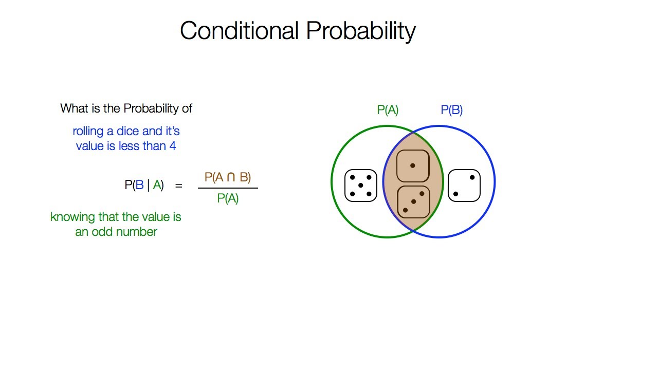
The following examples always refer to throws with a fair standard dice. The notation refers to an event that on a roll a one, a two or a three is rolled.

Special cases

General case

General is required in the Laplace experiment to calculate the conditional probability under the condition of the number of elements of the intersection

The event, at least a four (ie 4 or higher) to throw a priori probability.

Now, if it is known that an even number is rolled, that so the event has occurred, then there is the conditional probability for the condition due to

The conditional probability is greater than the output probability in this case.

If an odd number is rolled, that the event has occurred, the conditional probability for the condition is due to the same

The conditional probability in this case is smaller than the a-priori probability.

The event has a priori probability. If we know that the event has occurred, the probability due to changes in

Also in this example, the event is less likely due to the occurrence of the event, i.e., the probability that the event has occurred by the pitch has become small compared to the a priori probability as determined by the pitch, the event is any event occurred.

Trap

An illustrative example is to understand conditional probabilities based on quantity charts immediately allowed. Consider a throwing machine (eg, balls, darts ) on a given surface (eg a wall ) throws in a random manner any objects so that each place of the wall is made with equal probability. The function assigns the area or a specific partial area of ​​the wall (for example, any selected with a pin code), or to its surface area. Then the probability that the projectile impacts in proportional to the ratio of the partial area to the total, ie.

Now, it is also assumed that the projectile has struck within another sub-area that overlaps with the part surface. Then the probability that the missile strikes in. The conditional probability that the floor under the additional condition is incident at the same time within the overlapping sub-area is proportional to the surface area of that part of the surface which lies in, that is, the area of ​​the intersection. Conversely, for an equal failing intersection, the less likely that an incident at incident projectile in the greater was assumed. Is therefore inversely proportional.

Thus, the probability of incidence results in in addition vorausgesetztem impact in the conditional probability, so by definition.

Other examples

• For example, the conditional probability P ( "the earth is wet " | " it's raining ") (the soil is wet when it rains ) usually large, because under the condition that it is raining at a time, one should expect that the earth is wet. Conditional probability asks so after how likely an event is if I already know another. In our example, I know that it is raining, and I wonder how likely it is that the soil is wet. Obviously differs, the conditional probability of the unconditional.

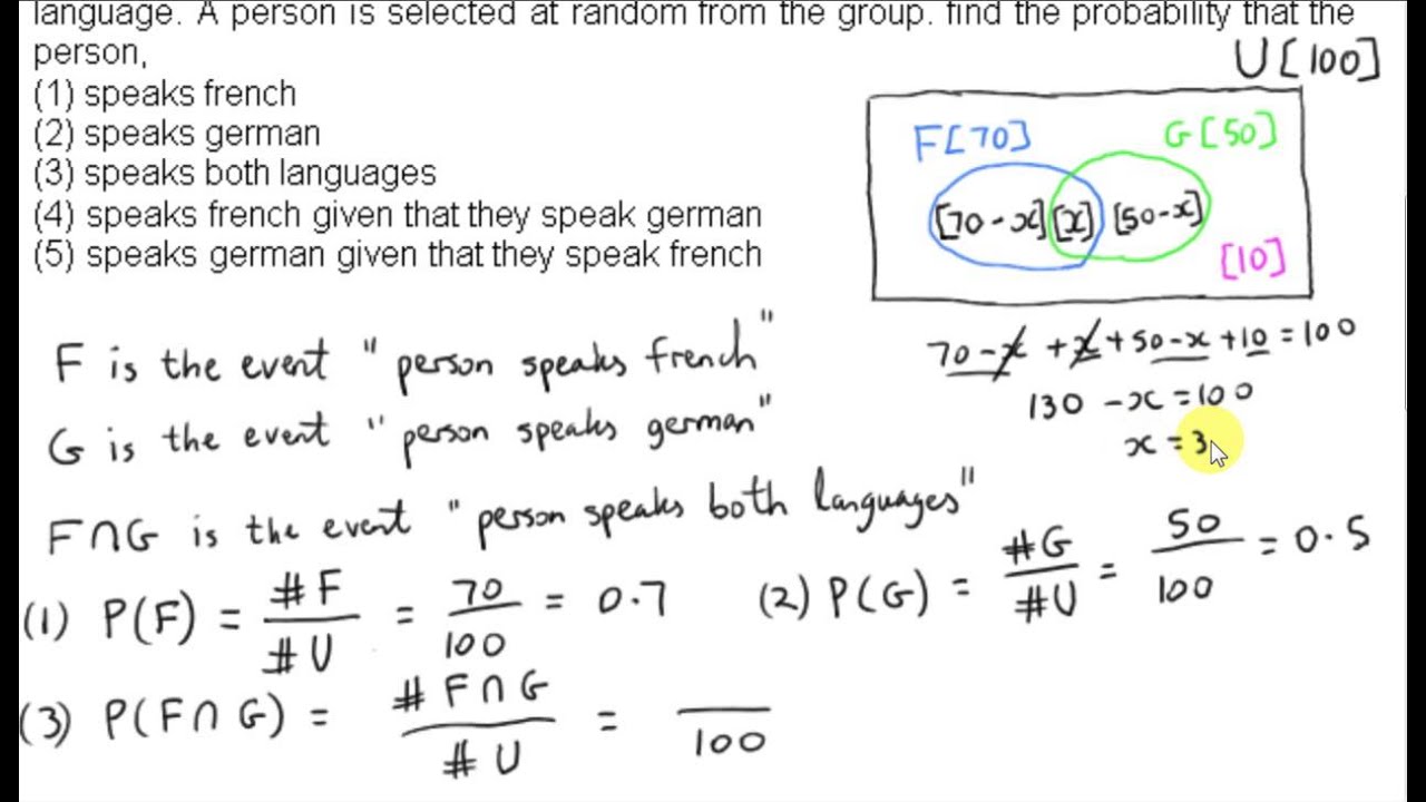
• The probability that someone who speaks French, a Frenchman is, is neither equal to the probability that someone who is a Frenchman who also speaks French, nor the two probabilities add up to 100 %.

• People v. Collins ( 1968): In this criminal trial in California a supposed male bank robber was sentenced, among other reasons, because the offender was under witness statements a beard and a mustache. Who has a beard, very often also has a mustache - the court went into his misjudgment but not from conditional probabilities.

• Draws in the sport: In 2013, there were two German and two Spanish teams in the semifinals of the Champions League. The probability that a purely German and an all-Spanish semi-final will be drawn in this constellation, is one-third, not fifty percent. Wanted is the probability that the second German ( Spanish ) association is drawn as a second club, under the condition that a German (Spanish ) Team was pulled from the Lostopf the first team. But if a German (Spanish ) club has been considered as first team, one of three remaining teams in the lottery wheel is just too German. Therefore, the required probability 1/3.